FIG. 01
RECORD DATA
Category
Software
DATE
Training finished and the terminal printed its final line: mAP50 0.950. There was a short burst of celebration on the team. The following week we flew the same model in the field and could not lock onto one of the targets no matter what we tried.
That contradiction gave us a reflex: stop trusting the metric. But that is the wrong reaction. The metric was not lying; we were asking it the wrong question. mAP50 0.950 does not say "the model works well in the field." It says "on these images, in this validation set, at an IoU threshold of 0.50, averaged across all confidence thresholds, precision is this." The distance between those two statements is as wide as the distance between flight day and a day at the office.
In this post we open up the detection metrics along with their formulas: which number measures what, when each one misleads you, and what we watch for in our own validation set.
First, IoU: when does a detection count as "correct"?
In classification, correctness is simple: the label either matches or it does not. In detection, the model also draws a box. Is the box in the right place? That is what IoU (Intersection over Union, the ratio of the overlap to the combined area) measures:
IoU= Area(prediction ∩ ground truth) / Area(prediction ∪ ground truth)
IoU runs between 0 and 1. A 1 means perfect overlap, a 0 means no overlap at all. You pick a threshold, typically 0.50, and sort the predictions into three groups:
Abbreviation | Name | What it means |
|---|---|---|
TP | True Positive | Correct class and IoU ≥ threshold |
FP | False Positive | Wrong class, or IoU < threshold, or a box produced where there is no object at all |
FN | False Negative | An object that is really there but the model failed to find |
Note what is missing from that list: there is no TN (True Negative). In detection you cannot count "background correctly not detected," because an image contains an unbounded number of boxes that are not objects. That is why accuracy is not used in detection: its denominator is undefined.
Precision and recall: two questions that push against each other
Two metrics fall out of the TP/FP/FN triple. Each one answers a single-sentence question:
Precision= TP / (TP + FP) → "How many of the things I found are actually correct?"
Recall= TP / (TP + FN) → "How many of the things that exist was I able to find?"
F1= 2 · (P · R) / (P + R) → the harmonic mean of the two
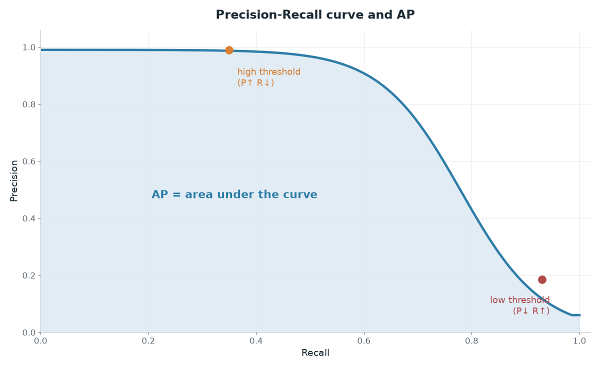
The two generally work against each other. Make the model bolder (a low confidence threshold) and recall rises while precision falls. Make it more cautious and the reverse happens.
Which one carries more weight depends on the mission. For our SUAS mission, the split looks like this:
Error type | What it looks like in the field | Cost |
|---|---|---|
FP (false detection) | An autonomous drop on a target that is not there | High: it costs points directly |
FN (missed target) | Flying over the target without dropping | Medium: the lap can be repeated |
So for us, precision is a little more expensive than recall. An autonomous drop decision cannot be taken back. That preference directly determined the confidence threshold we describe further down.
The PR curve, AP, and mAP
Precision and recall are not single numbers; they are functions of the confidence threshold. Sweep the threshold from 0.99 down to 0.01 and you get a curve: the precision-recall (PR) curve. The closer it hugs the top-left corner, the better.
AP (Average Precision) is the area under that curve. The COCO protocol, the method Ultralytics uses as well, computes it with 101-point interpolation: the recall axis is sampled at {0, 0.01, ..., 1.00}, at each point the maximum precision corresponding to that recall is taken, and the average is integrated.
AP= ∫₀¹ p(r) dr ≈ (1/101) · Σ p_interp(r), r ∈ {0.00, 0.01, ..., 1.00}
mAP= (1/N) · Σ AP_i (N = number of classes)
mAP (mean Average Precision) is then AP averaged over the classes. Our model has two classes, so mAP is the arithmetic mean of two APs; that detail matters, and we will come back to it shortly.
The difference between mAP50 and mAP50-95
In the definition above we fixed the IoU threshold at 0.50. That is mAP50. mAP50-95 is the average of the mAP values you get by sweeping the IoU threshold from 0.50 to 0.95 in steps of 0.05 (10 different thresholds):
mAP50-95= (1/10) · Σ mAP@IoU_t, IoU_t ∈ {0.50, 0.55, ..., 0.95}
In practice, here is what separates them:
Metric | What it measures | When to look at it |
|---|---|---|
mAP50 | "Did you find the object roughly in the right place?" | Detect-and-go tasks, where an object present/absent decision is enough |
mAP50-95 | "How accurate are the boundaries of the box?" | When you need precise localization, measurement, tracking, or a drop-point calculation |
mAP75 | Middle ground; strict, but not as brutal as 0.95 | When you are hunting down where the gap between the other two metrics comes from |
mAP50 is always higher than mAP50-95. If the gap between them is large, your model is finding the object but not seating the box properly on it. That gap typically widens on small objects: a shift of a few pixels drops IoU proportionally much further on a small box.
One warning: reporting mAP50 on its own makes the number look better than it is. We measured 0.950 for mAP50 on our own aerial-only validation set, and we always write that number with the qualifier "on the aerial-only validation set." Leave the qualifier off and the reader takes it for a claim about general capability.
Reading the confusion matrix
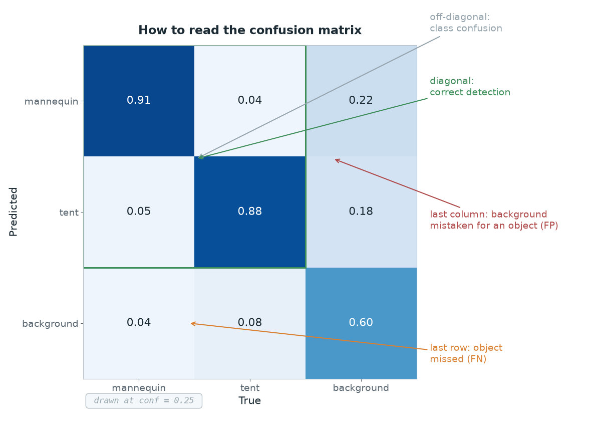
At the end of validation, Ultralytics plots a confusion matrix of size (nc+1) × (nc+1), where nc is the number of classes, and the extra row/column is background. That extra row is not a class the way it would be in a classification problem; it is a drain that collects unmatched predictions and missed ground-truth objects.
Cell | What it means | What to do |
|---|---|---|
Diagonal (class i → class i) | Correct detections | Nothing to do |
Class i → class j (off-diagonal) | Class confusion | Check label quality and visual similarity between the classes |
background → class i column | Mistook background for an object (FP) | Add hard negative samples, raise the threshold |
class i → background row | Missed a real object (FN) | Look at sample count, resolution, tiling |
One important detail: unlike the PR curve, the confusion matrix is plotted at a single confidence threshold, 0.25 by default in Ultralytics (as of 2026). So the matrix answers the question "what is the model doing at this threshold," while mAP is a summary across all thresholds. When the two disagree, look at the threshold first.
The confidence threshold: you are the one choosing the balance
A model does not arrive with a single threshold. That is also where the difference between the val and predict defaults comes from, and it confuses people regularly (as of 2026):
Argument | val default | predict default | Note |
|---|---|---|---|
| 0.001 | 0.25 | Deliberately very low in val, so that the whole PR curve comes out |
| 0.7 | 0.7 | This is the NMS threshold, not the ground-truth matching threshold |
| 300 | 300 | Maximum detections per image |
val using conf=0.001 is deliberate: it wants the curve to stretch all the way into the low-precision region. For that reason, do not mistake the precision/recall numbers in the validation output for the performance of your flight configuration. In flight we use conf=0.25; the real precision/recall at that threshold is a single point on the PR curve, not the row printed in the table.
Ultralytics also searches for the threshold that maximizes F1 on its own; the relevant line in the source is this:
In other words, the F1 curve averaged over the classes is lightly smoothed and its peak is located. That peak in the F1_curve.png output is a good starting point, but F1 weights precision and recall equally. On a mission like ours, where an FP is more expensive, picking a threshold slightly above the F1-optimal one is the rational move.
Common traps: four situations where the metric misleads you
1. A small validation set. On a set holding 40 objects, a difference of 2 detections can swing mAP by several points. Mistaking that noise for a real improvement is the easiest way to lock in a change that actually does nothing. Before you look at the number, look at how many objects are in the set.
2. Imbalanced classes. mAP averages the classes' APs with equal weight; it does not care about sample counts. In a two-class model, if the well-represented class scores 0.98 and the sparse one scores 0.62, mAP comes out at 0.80, and looking at that one number gives no hint that the second class has collapsed. Our own first dataset had a serious sample-count imbalance between the classes, which is why we made a habit of checking per class with metrics.box.maps.
3. Leaky validation (data leakage). This is the sneakiest one. If you randomly split consecutive frames pulled from the same video into train/val, the frame in the validation set is very nearly a copy of the one in training. The model memorizes, mAP goes up, field performance does not change. The correct unit of splitting is not the frame but the capture session: every frame from the same flight has to stay on the same side.
4. The wrong domain. If the validation set does not resemble the mission, the metric is measuring a different problem. Our first dataset was dominated by ground-level images scraped from the web, whereas the mission comes from a nadir-pointing camera hundreds of meters up. So we built the validation set from aerial footage only. The number went down, but its meaning went up.
All four collapse into a single sentence: mAP also measures how hard your dataset is. Pick an easy set and you get an easy number.
Practical summary
Do not report a single number. Write mAP50, mAP50-95, and per-class AP together; the gap between the first two gives you free information about your box accuracy.
Write the qualifier next to the metric. "mAP50 0.950 on the aerial-only validation set" and "mAP50 0.950" are different claims. Do not write the second one.
Split the validation set by session, not by frame. Frames from the same flight should never end up in both train and val.
Pick your flight threshold from the F1 curve, but shift it according to the mission's cost of error. On a mission where a false detection is expensive, a little above the F1 optimum is safer.
When mAP goes up, first check how many objects are in the set. The improvement you see on a small set is usually noise.
A metric is not the model's report card; it is the answer to the question you asked. Frame the question well and there are fewer surprises on flight day.