Perception

1 Scope and Mission Drivers

This document describes the perception stack of the Atılım UAV Team: the imaging hardware, the object detection pipeline, the aerial mapping pipeline, the simulation environment used for integration testing, and the target geolocation chain that connects a detection in image space to a delivery waypoint in the world frame.

Two SUAS 2026 mission elements drive every design decision below. Risk Mapping requires a georeferenced orthomosaic of the search area. Search-Detect-Deliver requires the UAS to find one mannequin and one open pop-up tent inside the search boundary and to deliver a water bottle to the mannequin and a strobing beacon to the tent, all while remaining above the 150 ft AGL floor.

Those two requirements set what follows: the altitude the optics are sized for, the choice of camera, and the split of compute between aircraft and ground station.

2 Imaging Hardware and Compute

The first question we answered was whether a target could physically be resolved at the planned mission altitude. SUAS enforces a 150 ft AGL (45.7 m) floor, and our mission altitude is set at 50 m (164 ft) AGL, comfortably above that floor; every optical decision below is sized around that 50 m nadir geometry.

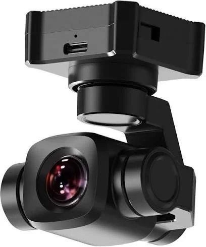
The camera is a SIYI A8 mini 3-axis gimbal unit, shown in Figure 1. It carries a 1/1.7 in Sony sensor with 8 MP effective resolution, a fixed 21 mm equivalent lens at F2.8, and an 81° horizontal / 93° diagonal field of view; it weighs 95 g and draws 5 W average [7]. It outputs over Ethernet, and that Ethernet output is what lets us pull two independent streams at once — the reason this unit beat the alternatives on our list.

2.1 Ground footprint and pixels on target at the 50 m mission altitude

At the 50 m mission altitude and the A8 mini's 81° horizontal FOV, unity zoom covers roughly 85 m of ground width in a single frame — wide enough that a full-boundary Risk Mapping survey needs only about 15–20 frames — while a 3x digital zoom, achieved by cropping the 4K sensor, narrows that FOV for detection and terminal guidance. Dividing the ground footprint by the output resolution gives the ground sample distance, and multiplying by the physical size of a target gives the number of pixels the target will span. In general, for a frame of width N_h pixels at height h above the target plane,

W_ground = 2h tan(HFOV / 2), GSD = W_ground / N_h (1)

Table 1 works Equation 1 through for both zoom settings at the 50 m mission altitude.

Table 1. Ground sample distance and pixels on target at 50 m nadir, for the A8 mini's unity and 3x digital zoom settings. Unity zoom is too coarse for reliable mannequin detection; the 3x setting used for detection and terminal guidance is what constrains the design.

Setting	Resolution / HFOV	GSD @ 50 m	Mannequin (~1.7 m)	Tent (~2.0 m)
Unity zoom (mapping)	1920 × 1080, 81° HFOV	44.5 mm/px	~38 px	~45 px
3x zoom (detection / terminal guidance)	1920 × 1080, 31.8° HFOV	14.8 mm/px	~115 px	~135 px

The conclusion we drew from Table 1 shaped the whole pipeline. At unity zoom a mannequin is only about 38 pixels across — too coarse for reliable detection, and that assumes the mannequin is fully exposed rather than partially occluded by bushes or vehicles, which the SUAS handbook explicitly warns it may be [1]. The 3x zoom setting brings that up to roughly 115 pixels, which is why it is the setting used operationally for detection and terminal guidance.

This GSD gap between zoom settings is a deliberate design choice, not a compute trade-off: unity zoom is used for the Risk Mapping survey, where wide ground coverage matters more than fine resolution, while the 3x setting is reserved for detection and terminal guidance, where target size on the frame is what matters.

The 50 m figure above is the mission altitude the detector and dataset are sized for. Field validation, described in Section 7, was first flown at 20 m AGL as a deliberate safety and logistics choice for early trials, and was then repeated at the full 50 m mission altitude with comparable detection confidence and delivery accuracy. Both altitudes fall comfortably inside the resolvable range Table 1 implies at 3x zoom.

2.2 Compute and link

Detection runs on an NVIDIA Jetson Orin NX 16 GB carried on the aircraft. Video reaches the ground station through the SIYI HM30 link, which also carries the MAVLink telemetry stream. Flight control is a Cube Orange Plus, paired with a CUAV Neo3 Pro GNSS receiver; the Neo3 Pro is a standalone receiver by design — the system does not depend on RTK or a ground-correction link, so waypoint navigation and release positioning stay available without one. Mission Planner is the ground control station used. Table 2 lists what each element contributes to perception.

Table 2. Perception hardware chain and the role each element plays. The flight controller and the GNSS receiver appear here only as pose and position sources, but they supply two of the five inputs the geolocation transform in Section 6 needs.

Component	Selection	Role in the perception stack
Camera / gimbal	SIYI A8 mini	Stabilized nadir RTSP imagery
Video link	SIYI HM30	Live operator video and MAVLink telemetry transport
Onboard compute	Jetson Orin NX 16 GB	Real-time YOLO11m inference, MAVLink command issue
Flight controller	Cube Orange Plus	Attitude, heading and navigation reference for geotagging
GNSS	CUAV Neo3 Pro (standalone)	Standalone aircraft position for target geolocation, no ground-correction link required
GCS	Mission Planner	Mission upload, telemetry, operator supervision

A single RTSP stream from the A8 mini is distributed by an onboard SwitchBlox network switch to both destinations: the Jetson, which processes only the most recent frame to avoid queue latency for detection, and the ground station over the HM30 link, which feeds the operator's live picture and the FastMosaic mapping pipeline. Codec is H.265 — H.264 was tried first and produced an unstable stream.

3 Object Detection

Before choosing a model we reviewed the Technical Design Reports of teams that competed at SUAS 2025 and compared what they used, what data they trained on, and whether their pipeline ran in real time. Table 3 summarizes that survey; of the five reports, the Alexandria University one [2] is the only one we hold a full citation for.

Table 3. Detection approaches reported by teams at SUAS 2025, as stated in their own Technical Design Reports. Every entry reported as real-time is a YOLOv11 variant; the two entries that are not real-time are the RF-DETR and DINOv2 + DETR pipelines.

Team	Model	Dataset	Real-time	Trade-off
Alexandria Univ.	RF-DETR	100% synthetic	No	Strong on small objects, expensive to train
Ohio State	DINOv2 + DETR	Real + synthetic	No	Highest mAP, highest latency
King Fahd Univ.	YOLOv11	AirSim + real	Yes	Balanced FPS/accuracy, loses detail on downscale
Hacettepe (Markut)	YOLOv11	30% synth + 70% real	Yes	Generalizes well, less sophisticated
KAAN Tech	YOLOv11m	COCO + task objects	Yes	Low cost, weaker localization

We selected YOLO11m, specifically the medium variant. The deciding factors were real-time capability on an embedded target, an acceptable FPS/accuracy balance, and by far the widest availability of tooling, export paths and community material — which matters for a student team that has to debug quickly [3]. Initial experiments showed that the limiting factor on performance was dataset diversity rather than network capacity, which is what shaped the data-generation work in Section 3.1 rather than a push toward a larger model. A P2 detection head and a dual-model ensemble were both evaluated as alternatives and rejected: neither justified its extra computational cost for a two-class detection problem.

3.1 Dataset

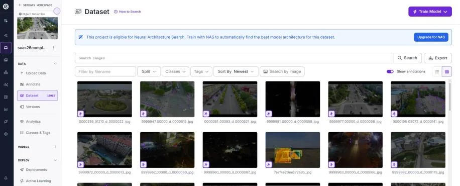
The dataset is managed in Roboflow and currently holds 16,015 images across the two mission classes, mannequin and tent. It is assembled, not just collected: multiple Roboflow projects were merged, duplicate images were removed by filename and perceptual-hash comparison, and fifteen original source classes were consolidated down to the two we need. Vehicle-related classes were discarded outright, and the resulting imbalance between mannequin and tent samples was reduced by oversampling tent images. It draws on three kinds of source imagery: public aerial imagery that supplies scale, viewpoint and background diversity; our own drone footage of mannequins captured over campus and park terrain; and close-range studio images of mannequins that anchor the object appearance. Figure 2 shows the project as it currently stands.

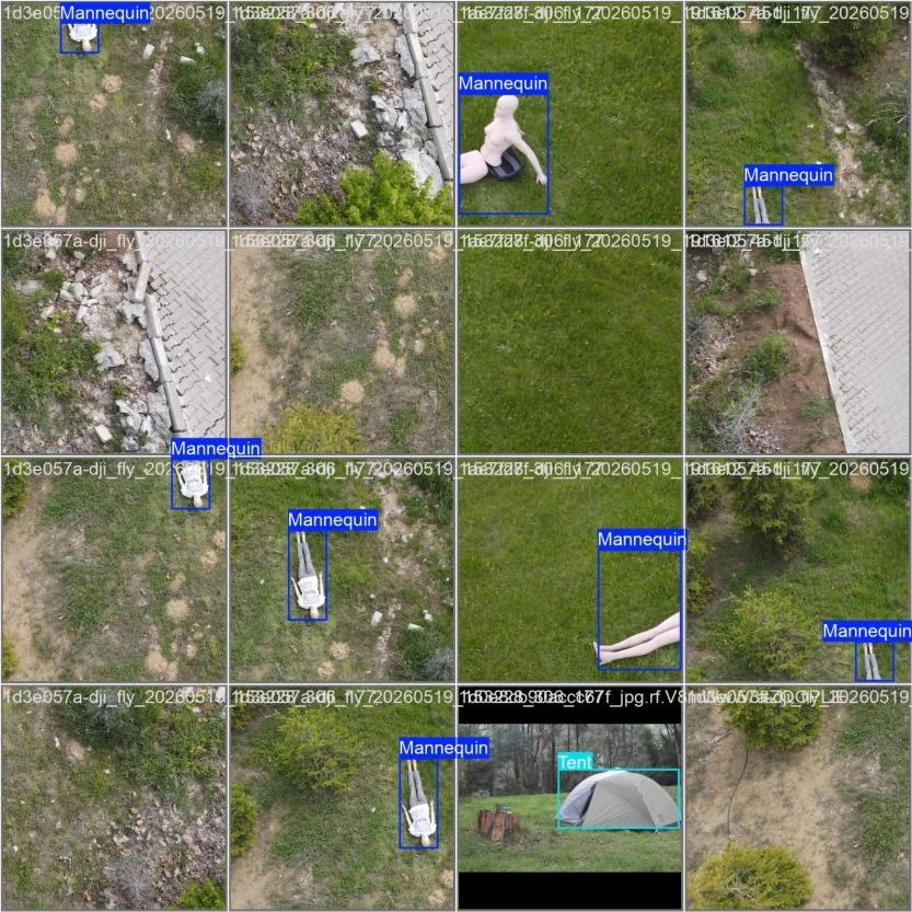
The real-image capture campaign was flown on 19 May 2026. Mannequins were placed on grass, gravel, paving and bare soil, in the poses the handbook says to expect — lying down, seated, face-down — and were photographed at competition-representative altitude so that the apparent target size in training matches the apparent target size at competition. Partial occlusion cases were captured deliberately: legs visible under a bush, torso only, mannequin next to debris. Figure 3 is a sample of the labeled result.

3.2 Training

Labeling was done in Label Studio and Roboflow. Training data are generated as overlapping 1280 × 1280 image tiles, together with hard-negative background tiles drawn from debris and grass environments so the model sees confusable clutter with no target in it. The model is initialized from COCO-pretrained weights at a 1280 px input resolution and fine-tuned on the custom set, with scaling, flipping, rotation, mosaic augmentation and mixup reintroduced during training to improve robustness to object scale and viewing angle. Validation is performed exclusively on real aerial DJI imagery rather than on held-out web imagery, so the reported metrics reflect the operational environment rather than the training distribution.

Table 4. Validation performance of the retrained YOLO11m model by class, on a validation set of 31 real aerial DJI images (121 labeled instances). The tent row is reported on only 6 validation instances and should be read with that in mind.

Class	P	R	mAP50	Val. instances
Mannequin	0.902	0.801	0.906	115
Tent	0.942	1.000	0.995	6
All	—	—	0.950	121

Overall mAP@50 is 0.950 and mAP@50–95 is 0.745; precision and recall are computed in the usual way, P = TP / (TP + FP) and R = TP / (TP + FN). Tent detection looks excellent, but six validation instances is too small a sample to claim statistical confidence beyond what is reported here — growing that validation set is tracked in Section 8. Tiled inference was also evaluated as a proof of concept for small-object recovery: on two held-out aerial images where full-frame inference produced no detections, tiled inference recovered 5 and 1 additional detections respectively, at a peak confidence of 0.74 — but onboard processing performance fell short of what autonomous guidance requires. TensorRT-accelerated tiled inference is therefore kept available only as a contingency configuration for smaller or lower-confidence targets, while the operational flight configuration — full-frame inference at 640 px with a 0.25 confidence threshold — is what the aircraft flies.

3.3 Validation on unseen footage

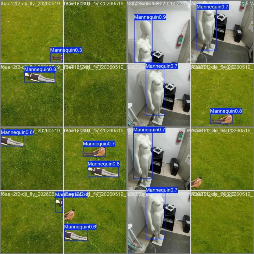
The model is validated on drone footage that was never part of training. Confidence on clearly exposed mannequins sits in the 0.6–0.9 band; heavily occluded or partially framed targets fall to 0.3, and some fully occluded instances are missed entirely. Figure 4 shows both ends of that range on one sheet.

One failure mode in this path is more serious than low confidence. The mannequin-only model has classified real humans as mannequins in earlier runs. Judges and other personnel may be inside the search boundary during a mission, so a false positive on a human would send a delivery toward a person rather than a target. Three mitigations are in progress: adding a human negative class to the dataset, keeping human-containing frames as hard negatives, and gating the delivery decision on a confidence threshold plus multi-frame agreement rather than on a single detection.

4 Mapping

The Risk Mapping task requires a single stitched image of the search area, generated on site immediately after the survey and written directly in the submission-ready format. Our in-house mosaicker, FastMosaic (organized under the suas_fast_orthomosaic project), is built for that specific job: fast on-site turnaround, robustness to the small frame count of a single survey pass (15–20 frames), and visual consistency across frame seams, rather than general-purpose photogrammetry.

FastMosaic runs in four stages. GPS-assisted frame selection orders frames by the flight log and gates out any frame taken during a sharp maneuver (heading change greater than 30°). Each remaining frame is matched against a sliding buffer of recent frames using ORB features with CLAHE contrast normalization [5], and placed with a 4-degree-of-freedom similarity transform estimated by RANSAC,

x′ = s R(θ) x + t (2)

Distance-transform feathering, with blend weight w = d_new / (d_new + d_old), merges each frame into the canvas, which is then cropped and written directly as the PNG the rules require. GPS is used for selection and sequencing while the actual placement is computed from visual features — geotags alone cannot give pixel-level alignment, and features alone cannot give ordering robustness, so the pipeline uses each source for what it is good at.

We built FastMosaic in house rather than adopting an external photogrammetry suite such as OpenDroneMap [6] to keep the mapping chain under end-to-end control inside the same Python toolchain as the rest of the software, avoid an external processing dependency at the field station, and produce the submission PNG directly. It also runs a mode batch photogrammetry tools do not: a real-time preview that consumes the A8 mini’s RTSP stream during the survey itself, so a coverage gap costs a re-fly of one leg rather than a hole discovered later in the submitted map.

The output is a visual mosaic rather than a rigorously orthorectified product: the similarity transform in Equation 2 does not model perspective or terrain relief, and incremental placement can accumulate drift over long chains. We control quality at the source instead — nadir gimbal imagery, an overlap-rich survey pattern and the maneuver gate — and validate it by side-by-side comparison against reference imagery of the same area. Camera intrinsics currently use nominal datasheet values (fx ≈ 1124 px) and lens distortion is uncorrected; a checkerboard calibration is the planned refinement once physical camera access allows.

Mapping is executed on the ground station using the same RTSP stream distributed by the SwitchBlox switch, which keeps the Jetson free for detection. This follows directly from the single-stream architecture described in Section 2.2.

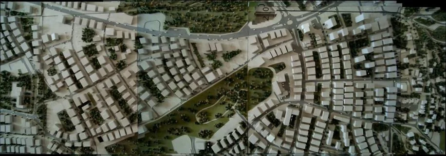
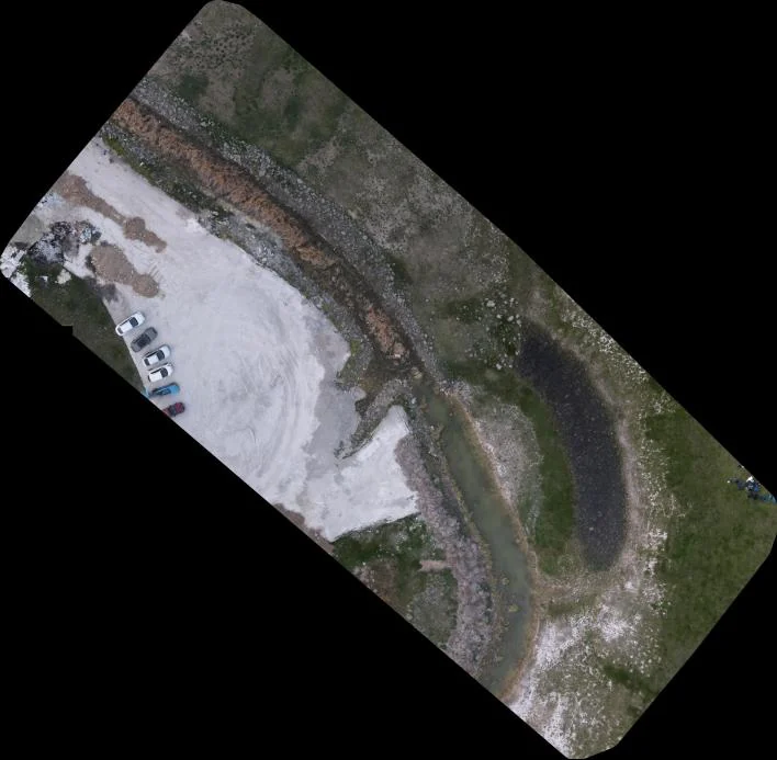
Two early stitching tests are shown below. Figure 5 is the first, over a scale model; Figure 6 is the second, over the flight-test field.

4.1 Test status

Mapping has been verified at both the component and mission level. Before flight operations, RTSP video ingestion from the SIYI A8 mini was validated with a dedicated bench-testing utility. During map generation, frames captured during sharp heading changes are filtered automatically, and frames that fail feature matching are discarded rather than forced into the final mosaic, which is what keeps overall map quality up.

The resulting mosaic was evaluated against the SUAS mapping requirements directly: complete coverage of the surveyed area, seamless alignment with no visible stitching artifacts, consistent exposure across the mosaic, and visual comparison against reference imagery of the same region. All four criteria were met, which is what makes the current pipeline competition-ready rather than a proof of concept. Georeferencing the output — turning the visual mosaic into a coordinate-accurate product rather than a visually consistent one — remains future work and is tracked in Section 8.

5 Simulation

We put a deliberate emphasis on integration testing in simulation this year, so that time in the field is spent flying rather than debugging: every new capability is flown in simulation before it is flown on hardware.

The environment brings together Gazebo, ArduPilot SITL, ROS 2 and pymavlink, and it is built to reproduce the actual flight architecture rather than run as a single desktop process — the flight-dynamics simulator, the Mission Planner ground station and the Jetson companion computer run as separate nodes on a shared network. Camera imagery reaches the Jetson over the same RTSP stream a real flight would use, so the full image-processing pipeline runs under conditions that closely match hardware. This is what shortens iteration time and keeps early testing risk off the airframe.

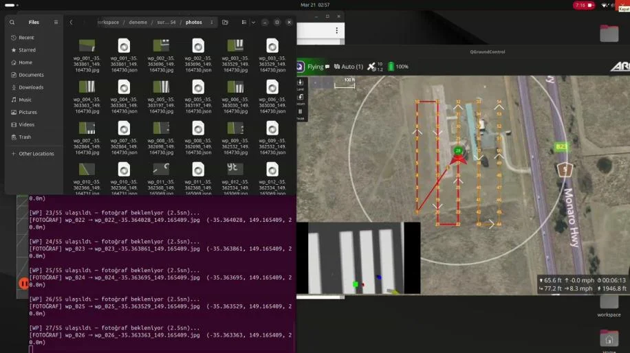
Flight-path testing uses SITL and Gazebo for autonomous takeoff, waypoint navigation, landing and Return-to-Launch scenarios, with missions planned and monitored in Mission Planner and survey grids generated with the Simple Grid tool. PID tuning and GPS-lock logic are validated against a simulation model configured with the weight and propeller characteristics of the actual platform (MN505), so flight-controller behavior is checked before it reaches hardware. The scenario in Figure 7 is one such run, a 55-waypoint survey mission. At each waypoint the vehicle holds, the capture routine triggers, and the frame is written to disk with the capture position encoded in the filename and a JSON sidecar carrying the full pose — exactly the geotagged image set the mapping pipeline consumes, produced without requiring a flight.

Object detection is exercised in simulation too: simulated targets with known positions and orientations are placed in the Gazebo world so that detection accuracy, bounding-box alignment, processing latency and the resulting geolocation can be checked against ground truth before they are trusted on the target hardware.

Emergency scenarios — GPS/EKF degradation, communication loss with the ground station or the Jetson, and low-battery conditions — are injected through SITL, and the resulting automatic LOITER, landing and Return-to-Launch behaviors are verified through telemetry logs; the networked-node architecture also makes it possible to test communication latency and link interruptions realistically rather than simulate them abstractly.

MAVLink command handling is tested in the same environment: GUIDED mode entry, arm, autonomous takeoff to a set altitude, waypoint navigation, controlled landing and disarm. Commands are signed [4]. One defect is open against that signing implementation: during SITL testing we observed that a connection could in some cases be accepted even when an incorrect signing key was presented. This is a security defect in our implementation, it is under investigation, and it is tracked as open.

Simulation results do not transfer unconditionally, and two classes of measurement are treated as untrustworthy until re-taken on the target hardware. Gazebo holds roughly a 1.0 real-time factor on the development PC but drops to about 0.4–0.7 on the Jetson Orin NX under load, which distorts control-loop behavior. Inference FPS measured on a desktop GPU likewise does not predict Jetson performance; TensorRT FP16/INT8 export changes it by 2–4×. Development iterates on the PC; every latency-critical result is re-validated on the Jetson before it is trusted.

6 Target Geolocation

Detection alone does not complete the mission. The output of the detector is a bounding box in image coordinates; the delivery system needs a latitude and longitude. The module that converts one into the other is the link between perception and action.

Because the gimbal holds the camera at nadir and absorbs aircraft roll and pitch, a target pixel (u, v) in a W × H frame already defines a ray expressed in a locally level forward-right-down frame; it is brought into the local NED frame by the aircraft heading ψ alone, as reported by the flight controller:

r_c = [ −(v − H/2) / (H / (2 tan(VFOV/2))), (u − W/2) / (W / (2 tan(HFOV/2))), 1 ]^T, r_n = R(ψ) r_c (3)

Intersecting that ray with the ground plane at the known AGL altitude h gives the north and east offsets of the target, and from there its coordinates, with latitude and longitude in radians and R_E the local Earth radius:

[ΔN, ΔE]^T = (h / r_D) [r_N, r_E]^T, lat_t = lat + ΔN / R_E, lon_t = lon + ΔE / (R_E cos(lat)) (4)

Equations 3 and 1 are two views of the same pinhole model: the per-pixel scale 2 tan(HFOV/2)/W in Equation 3 is the inverse focal length 1/f, with f = (W/2)/tan(HFOV/2) ≈ 1124 px, and the ground sample distance in Equation 1 is that same factor projected onto the ground, GSD = h/f. Detection sizing and target geolocation therefore rest on one camera model rather than two independent calibrations. The resulting coordinate is issued to the flight controller as a MAVLink waypoint [4].

6.1 Terminal guidance

A single logged coordinate carries the geolocation error of one detection, and the aircraft still has to be centered over the target at the instant of release. An implemented terminal-guidance stage closes that gap by switching from the stored coordinate to the live image once the aircraft has navigated to it and settled: an image-based visual servoing controller drives the image-plane offset of the detected target from the frame center, e = (e_u, e_v) = (u − W/2, v − H/2), to zero. The offset is smoothed with an exponential moving average (α = 0.15) to reject detection jitter, mapped onto the nadir camera’s body axes, and fed to a discrete PID law running at 20 Hz (Δt = 0.05 s) that produces body-frame velocity commands, rotated into the NED frame by the current yaw:

v_b[k] = Kp ē_b[k] + Ki Σ ē_b Δt + Kd ( ē_b[k] − ē_b[k−1] ), ē_b = [−ē_v, ē_u]^T, [v_N, v_E]^T = R(ψ) v_b (5)

The gains are Kp = 0.003 and Kd = 0.004 (m/s)/px with Ki = 0.0001 (m/s)/(px s); the integral term is clamped to prevent wind-up while the target is briefly occluded, and command magnitude is saturated at 0.8 m/s so the aircraft converges without overshoot. Because detections are reported in the full 1920 × 1080 frame, release is armed only once the target has stayed within 20 px of the frame center for a sustained period — 0.30 m on the ground at the 50 m mission altitude with 3x zoom, by Equation 1 — and a target lost for a sustained period aborts the approach back to the waypoint mission.

The controller currently uses a fixed-depth approximation that holds the estimated range at the release altitude rather than scaling gain with measured range, so as tuned it is only valid at that one altitude; a range-scheduled gain would be needed before operating it at a materially different one.

6.2 Chain status

Table 5 sets out the full chain from frame to release and where each stage currently stands. The field validation in Section 7 exercised capture through approach end to end, but the release there was still commanded from the stored geolocation alone — closing the terminal-guidance loop of Section 6.1 on the live image is the next milestone, tracked in Section 8.

Table 5. Detection-to-delivery chain, stage by stage. Every stage has now been exercised in an integrated flight test; terminal guidance is the refinement that still needs to close on the live image rather than the stored coordinate.

Stage	Input	Output	Status
Capture	A8 mini RTSP stream	Frame + timestamp	Working
Detection	Frame	Class + bounding box	Working
Geolocation	Box + pose + intrinsics	Target lat/lon	Working, field-validated
Command	Target lat/lon	MAVLink waypoint	Working
Approach (open-loop)	Waypoint	Navigate to stored coordinate + release	Working, field-validated
Terminal guidance (visual servoing)	Live frame offset	Closed-loop approach correction	Implemented, pending flight validation

Accuracy here is directly scoreable. SUAS awards 50 points for landing a payload within 50 ft of a target and a further 30 points for delivering the correct object to the correct target [1]. In the integrated flight tests at both the 20 m and 50 m mission altitude, both deliveries landed well inside that radius on the open-loop chain alone — Section 7 has the numbers — which is encouraging, but two flights are not a statistical guarantee, and the miss distance on the water-bottle drop is exactly the margin closing the terminal-guidance loop is meant to tighten.

7 Field Validation

Field validation proceeded in three stages: low-light detection robustness, detection confidence at the 50 m mission altitude, and full end-to-end missions.

7.1 Detection under low light

Detection robustness was evaluated under low-light conditions using human stand-ins positioned on concrete surfaces. Across six trials the detection system consistently produced confidence values of approximately 0.75 from distances of 20–25 m, despite environmental conditions that differed from the primary training dataset — a useful margin above the 0.25 confidence threshold the operational flight configuration uses.

7.2 Detection at mission altitude

With the aircraft at 49 m AGL and the camera at 3x zoom, a human stand-in was detected with confidence between 0.60 and 0.80 — above the 0.25 threshold the operational flight configuration uses.

7.3 End-to-end flight test

With the earlier stages passed, end-to-end flight tests validated the complete autonomous mission pipeline under real operating conditions. In the first test, flown at approximately 20 m AGL, both competition targets were detected, their positions were transferred to the guidance system, and autonomous navigation proceeded to the computed release locations without operator intervention: the strobing beacon landed successfully on the tent target, while the water bottle landed approximately 5 m from the mannequin. The test was then repeated at the full 50 m mission altitude, with comparable detection confidence and a comparable delivery offset. Both tests placed both payloads comfortably inside the 50 ft (15.2 m) scoring radius, and both were commanded from the stored geolocation alone — the terminal-guidance loop of Section 6.1 was not yet closed for either test, which is consistent with the water-bottle miss distance being the kind of error that loop is designed to remove.

8 Ongoing Work

The open items below follow directly from where each module currently stands: geolocation and delivery work end to end but are open-loop, tent-class validation is thin, the camera model is uncalibrated, mapping is visually but not geometrically accurate, and one security defect from simulation testing remains unresolved.

• Close the terminal-guidance loop of Section 6.1 on the live image, and validate it against the open-loop result from Section 7 on a repeat flight at the 50 m mission altitude.

• Range-scheduled gain for the terminal-guidance controller, so it is not tuned to the single 50 m mission altitude.

• Checkerboard calibration of the SIYI A8 mini to correct lens distortion in both the geolocation and mapping camera models, which currently use nominal datasheet intrinsics.

• Grow the tent-class validation set beyond its current 6 instances for a statistically meaningful mAP figure.

• Georeference the FastMosaic output so the Risk Mapping deliverable is coordinate-accurate rather than only visually consistent.

• Resolution and verification of the MAVLink signing vulnerability found during SITL testing.

References

[1] RoboNation, “SUAS 2025 Team Handbook,” 2025.

[2] Alexandria University, “Alex Eagles Technical Design Report,” SUAS 2025.

[3] Ultralytics, “YOLO11 Documentation.” [Online]. Available: https://docs.ultralytics.com

[4] MAVLink, “MAVLink Developer Guide.” [Online]. Available: https://mavlink.io

[5] E. Rublee, V. Rabaud, K. Konolige, and G. Bradski, “ORB: An efficient alternative to SIFT or SURF,” in 2011 International Conference on Computer Vision, 2011, pp. 2564–2571.

[6] OpenDroneMap Authors, “ODM: A command line toolkit to generate maps, point clouds, 3D models and DEMs from drone, balloon or kite images,” https://github.com/OpenDroneMap/ODM, 2020.

[7] SIYI Technology, “A8 mini User Manual v1.6,” 2024.